Important Information
This file has a lot of Latex and GitHub currently cannot render it on Markdown files. You can read all the math clearly as a webpage or access this as a regular github repository.
The source of this example can be found here and the output here.
See the top directory of this repository for instructions to set up the NAG Library for Java.
This example demontrates how to fit data to a model using weighted nonlinear least-squares.
handle_solve_bxnl (e04gg) is a bound-constrained nonlinear least squares trust region solver (BXNL) from the NAG optimization modelling suite aimed for small to medium-scale problems. It solves the problem:
where \(r_i(x),i=1,\dots,n_{\text{res}}\), are smooth nonlinear functions called residuals, \(w_i ,i=1,\dots,n_{\text{res}}\) are weights (by default they are all defined to 1, and the rightmost element represents the regularization term with parameter \(\sigma\geq0\) and power \(p>0\). The constraint elements \(l_x\) and \(u_x\) are \(n_{\text{var}}\)-dimensional vectors defining the bounds on the variables.
Typically in a calibration or data fitting context, the residuals will be defined as the difference between the observed values \(y_i\) at \(t_i\) and the values provided by a nonlinear model \(\phi(t;x)\), i.e., \(r_i(x)≔y_i-\phi(t_i;x).\)
The following example illustrates the usage of e04gg to fit PADC target with \(\alpha\) particle
etched nuclear track data to a convoluted distribution. A target
sheet is scanned and track diameters (red wedges in
the following Figure 1) are recorded into a histogram and a mixed Normal and log-Normal model is to be fitted to the experimental histogram (see Figure 2).
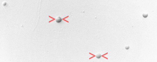
Figure 1: PADC with etched \(\alpha\) particle tracks.
e04gg is used to fit the six parameter model
\(\begin{array}{ll}
\phi\big(t, x = (a, b, A_{\ell}, \mu, \sigma, A_g)\big) = \text{log-Normal}(a, b, A_l) + \text{Normal}(\mu, \sigma^2, A_g)\\
\text{subject to } 0 \leq x,
\end{array}\)
using the histogram heights reported in Figure 2.
    // problem data
    // number of observations
    int nres = 64;
    // ovservations
    int[] diameter = new int[nres];
    for (i = 0; i < nres; i++) {
        diameter[i] = i + 1;
    }
    double[] density = new double[] { 0.0722713864, 0.0575221239, 0.0604719764, 0.0405604720, 0.0317109145,
            0.0309734513, 0.0258112094, 0.0228613569, 0.0213864307, 0.0213864307, 0.0147492625, 0.0213864307,
            0.0243362832, 0.0169616519, 0.0095870206, 0.0147492625, 0.0140117994, 0.0132743363, 0.0147492625,
            0.0140117994, 0.0140117994, 0.0132743363, 0.0117994100, 0.0132743363, 0.0110619469, 0.0103244838,
            0.0117994100, 0.0117994100, 0.0147492625, 0.0110619469, 0.0132743363, 0.0206489676, 0.0169616519,
            0.0169616519, 0.0280235988, 0.0221238938, 0.0235988201, 0.0221238938, 0.0206489676, 0.0228613569,
            0.0184365782, 0.0176991150, 0.0132743363, 0.0132743363, 0.0088495575, 0.0095870206, 0.0073746313,
            0.0110619469, 0.0036873156, 0.0051622419, 0.0058997050, 0.0014749263, 0.0022123894, 0.0029498525,
            0.0014749263, 0.0007374631, 0.0014749263, 0.0014749263, 0.0007374631, 0.0000000000, 0.0000000000,
            0.0000000000, 0.0000000000, 0.0000000000 };

    // Define iuser and ruser to be passed to the callback functions
    int[] iuser = diameter;
    double[] ruser = density;
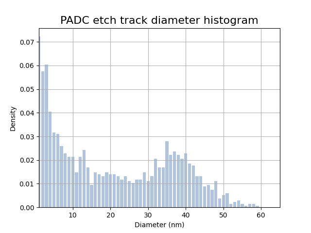
Figure 2: Histogram of etched track diameter of \(\alpha\) particles. Bar heights are the data that will be fitted unsing the aggregated model \(\phi(x, t)\).
    // Define Normal and log-Normal distributions
    public static double lognormal(int d, double a, double b, double Al) {
        return Al / (d * b * Math.sqrt(2 * Math.PI)) * Math.exp(-(Math.pow(Math.log(d) - a, 2)) / (2 * Math.pow(b, 2)));
    }

    public static double gaussian(int d, double mu, double sigma, double Ag) {
        return Ag * Math.exp(-0.5 * Math.pow((d - mu) / sigma, 2)) / (sigma * Math.sqrt(2 * Math.PI));
    }

    public static double[] lognormal(double[] d, double a, double b, double Al) {
        double[] result = new double[d.length];
        for (int i = 0; i < d.length; i++) {
            result[i] = Al / (d[i] * b * Math.sqrt(2 * Math.PI)) * Math.exp(-(Math.pow(Math.log(d[i]) - a, 2)) / (2 * Math.pow(b, 2)));
        }
        return result;
    }

    public static double[] gaussian(double[] d, double mu, double sigma, double Ag) {
        double[] result = new double[d.length];
        for (int i = 0; i < d.length; i++) {
            result[i] = Ag * Math.exp(-0.5 * Math.pow((d[i] - mu) / sigma, 2)) / (sigma * Math.sqrt(2 * Math.PI));
        }
        return result;
    }
In terms of solving this problem, the function to minimize is the sum of residuals using the model \(\phi(x;t)\)
and the data pair (diameter, density). The parameter vector is \(x = (a, b, A_l, \mu, \sigma, A_g)\). The next step is to define a function to return the residual vector
\(\text{lsqfun}(x) := \big[r_1(x), r_2(x), \dots, r_{n_{\text{res}}}(x)\big]\).
    // Define the least-square function as a mixture of Normal and log-Normal
    // functions. Also add its first derivatives

    /**
     * Objective function callback passed to the least squares solver. x = (a, b,
     * Al, mu, sigma, Ag)
     */
    public static class LSQFUN extends E04GG.Abstract_E04GG_LSQFUN {
        public void eval() {
            int[] d = this.IUSER;
            double[] y = this.RUSER;
            double a = this.X[0];
            double b = this.X[1];
            double Al = this.X[2];
            double mu = this.X[3];
            double sigma = this.X[4];
            double Ag = this.X[5];

            for (int i = 0; i < this.NRES; i++) {
                this.RX[i] = lognormal(d[i], a, b, Al) + gaussian(d[i], mu, sigma, Ag) - y[i];
            }
        }
    }

    /**
     * Computes the Jacobian of the least square residuals. x = (a, b, Al, mu,
     * sigma, Ag)
     */
    public static class LSQGRD extends E04GG.Abstract_E04GG_LSQGRD {
        public void eval() {
            int n = this.X.length;
            int[] d = this.IUSER;
            double a = this.X[0];
            double b = this.X[1];
            double Al = this.X[2];
            double mu = this.X[3];
            double sigma = this.X[4];
            double Ag = this.X[5];
            for (int i = 0; i < this.NRES; i++) {
                // log-Normal derivatives
                double l = lognormal(d[i], a, b, Al);
                // dl/da
                this.RDX[i * n + 0] = (Math.log(d[i]) - a) / Math.pow(b, 2) * l;
                // dl/db
                this.RDX[i * n + 1] = (Math.pow(Math.log(d[i]) - a, 2) - Math.pow(b, 2)) / Math.pow(b, 3) * l;
                // dl/dAl
                this.RDX[i * n + 2] = lognormal(d[i], a, b, 1.0);
                // Gaussian derivatives
                double g = gaussian(d[i], mu, sigma, Ag);
                // dg/dmu
                this.RDX[i * n + 3] = (d[i] - mu) / Math.pow(sigma, 2) * g;
                // dg/dsigma
                this.RDX[i * n + 4] = (Math.pow(d[i] - mu, 2) - Math.pow(sigma, 2)) / Math.pow(sigma, 3) * g;
                // dg/dAg
                this.RDX[i * n + 5] = gaussian(d[i], mu, sigma, 1.0);
            }
        }
    }
    // parameter vector: x = (a, b, Al, mu, sigma, Ag)
    int nvar = 6;

    // Initialize the model handle
    E04RA e04ra = new E04RA();
    long handle = 0;
    int ifail = 0;
    e04ra.eval(handle, nvar, ifail);

    handle = e04ra.getHANDLE();

    // Define a dense nonlinear least-squares objective function
    E04RM e04rm = new E04RM();
    ifail = 0;
    e04rm.eval(handle, nres, 0, 0, new int[] {}, new int[] {}, ifail);

    // Add weights for each residual
    double[] weights = new double[nres];
    Arrays.fill(weights, 1.0);
    for (i = 55; i < 63; i++) {
        weights[i] = 5.0;
    }
    double weights_sum = Arrays.stream(weights).sum();
    for (i = 0; i < weights.length; i++) {
        weights[i] /= weights_sum;
    }

    // Define the reliability of the measurements (weights)
    E04RX e04rx = new E04RX();
    ifail = 0;
    e04rx.eval(handle, "RW", 0, weights.length, weights, ifail);

    // Restrict parameter space (0 <= x)
    E04RH e04rh = new E04RH();
    double[] bl = new double[nvar];
    double[] bu = new double[nvar];
    Arrays.fill(bu, 100.0);
    ifail = 0;
    e04rh.eval(handle, nvar, bl, bu, ifail);

    // Set some optional parameters to control the output of the solver
    E04ZM e04zm = new E04ZM();
    ifail = 0;

    e04zm.eval(handle, "Print Options = NO", ifail);
    e04zm.eval(handle, "Print Level = 1", ifail);
    e04zm.eval(handle, "Print Solution = X", ifail);
    e04zm.eval(handle, "Bxnl Iteration Limit = 100", ifail);
    // Add cubic regularization term (avoid overfitting)
    e04zm.eval(handle, "Bxnl Use weights = YES", ifail);
    e04zm.eval(handle, "Bxnl Reg Order = 3", ifail);
    e04zm.eval(handle, "Bxnl Glob Method = REG", ifail);

    // Define initial guess (starting point)
    double[] x = new double[] { 1.63, 0.88, 1.0, 30, 1.52, 0.24 };
Call the solver
    // Call the solver
    E04GG e04gg = new E04GG();
    LSQFUN lsqfun = new LSQFUN();
    LSQGRD lsqgrd = new LSQGRD();
    LSQHES lsqhes = new LSQHES();
    LSQHPRD lsqhprd = new LSQHPRD();
    MONIT monit = new MONIT();
    double[] rx = new double[nres];
    double[] rinfo = new double[100];
    double[] stats = new double[100];
    long cpuser = 0;
    ifail = 0;

    e04gg.eval(handle, lsqfun, lsqgrd, lsqhes, lsqhprd, monit, nvar, x, nres, rx, rinfo, stats, iuser, ruser,
            cpuser, ifail);
 E04GG, Nonlinear least squares method for bound-constrained problems
 Status: converged, an optimal solution was found
 Value of the objective             4.44211E-08
 Norm of projected gradient         1.18757E-09
 Norm of scaled projected gradient  3.98428E-06
 Norm of step                       1.66812E-01

 Primal variables:
   idx   Lower bound       Value       Upper bound
     1   0.00000E+00    2.02043E+00    1.00000E+02
     2   0.00000E+00    1.39726E+00    1.00000E+02
     3   0.00000E+00    6.93255E-01    1.00000E+02
     4   0.00000E+00    3.65929E+01    1.00000E+02
     5   0.00000E+00    7.01808E+00    1.00000E+02
     6   0.00000E+00    3.36877E-01    1.00000E+02
The optimal solution \(x\) provides the unfolded parameters for the two distributions, Normal and log-Normal (blue and red curves in Figure 4). Adding these together produces the aggragated curve (shown in color green of Figure 3 and 4) this last one is the one used to perform the fitting with. The optimal solution is
    // Optimal parameter values
    // Al * log-Normal(a, b):
    double aopt = x[0];
    double bopt = x[1];
    double Alopt = x[2];

    // Ag * gaussian(mu, sigma):
    double muopt = x[3];
    double sigmaopt = x[4];
    double Agopt = x[5];
and the objective function value is
Objective Function Value: 4.4421102582032467E-8
The next plot in Figure 3 illustrates the mixed-distribution fit over the histogram:
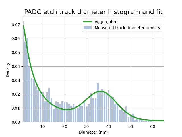
Figure 3: Histogram with aggregated fit.
The plot below in Figure 4 shows the unfolded fit, in red the log-Normal distribution and blue the Normal one:
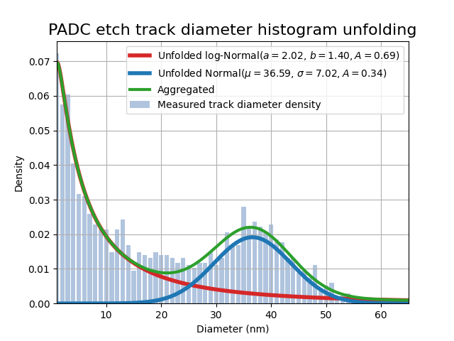
Figure 4: Aggregated model used for the fitting (green curve) and unfolded models (blue and red curves). Optimal parameter values are ported in the legend.
Finally, clean up and destroy the handle
    // Destroy the handle:
    E04RZ e04rz = new E04RZ();
    ifail = 0;
    e04rz.eval(handle, ifail);