Using DFO-LS
This section describes the main interface to DFO-LS and how to use it.
Nonlinear Least-Squares Minimization
DFO-LS is designed to solve the local optimization problem
where the bound constraints \(a \leq x \leq b\) and general convex constraints \(x\in C\) are optional. The upper and lower bounds on the variables are non-relaxable (i.e. DFO-LS will never ask to evaluate a point outside the bounds). The general convex constraints are also non-relaxable, but they may be slightly violated at some points from rounding errors. The function \(h(x)\) is an optional regularizer, often used to avoid overfitting, and must be Lipschitz continuous and convex (but possibly non-differentiable). A common choice is \(h(x)=\lambda \|x\|_1\) (called L1 regularization or LASSO) for \(\lambda>0\). Note that in the case of Tikhonov regularization/ridge regression, \(h(x)=\lambda\|x\|_2^2\) is not Lipschitz continuous, so should instead be incorporated by adding an extra term into the least-squares sum, \(r_{m+1}(x)=\sqrt{\lambda} \|x\|_2\).
DFO-LS iteratively constructs an interpolation-based model for the objective, and determines a step using a trust-region framework. For an in-depth technical description of the algorithm see the papers [CFMR2018], [HR2022] and [LLR2024].
How to use DFO-LS
The main interface to DFO-LS is via the function solve
soln = dfols.solve(objfun, x0)
The input objfun is a Python function which takes an input \(x\in\mathbb{R}^n\) and returns the vector of residuals \([r_1(x)\: \cdots \: r_m(x)]\in\mathbb{R}^m\). Both the input and output of objfun must be one-dimensional NumPy arrays (i.e. with x.shape == (n,) and objfun(x).shape == (m,)).
The input x0 is the starting point for the solver, and (where possible) should be set to be the best available estimate of the true solution \(x_{min}\in\mathbb{R}^n\). It should be specified as a one-dimensional NumPy array (i.e. with x0.shape == (n,)).
As DFO-LS is a local solver, providing different values for x0 may cause it to return different solutions, with possibly different objective values.
In newer version of DFO-LS (v1.6 onwards), the input x0 may instead by an instance of a dfols.EvaluationDatabase, which stores a collection
of previously evaluated points and their associated vectors of residuals. One of these points is designated the starting point for the solver, and the other
points may be used by DFO-LS to build its first approximation to objfun, reducing the number of evaluations required to begin the main iteration.
See the example below for more details for how to use this functionality.
The output of dfols.solve is an object containing:
soln.x- an estimate of the solution, \(x_{min}\in\mathbb{R}^n\), a one-dimensional NumPy array.soln.resid- the vector of residuals at the calculated solution, \([r_1(x_{min})\:\cdots\: r_m(x_{min})]\), a one-dimensional NumPy array.soln.f- the objective value at the calculated solution, \(f(x_{min})\), a Float.soln.jacobian- an estimate of the Jacobian matrix of first derivatives of the residuals, \(J_{i,j} \approx \partial r_i(x_{min})/\partial x_j\), a NumPy array of size \(m\times n\).soln.nf- the number of evaluations ofobjfunthat the algorithm needed, an Integer.soln.nx- the number of points \(x\) at whichobjfunwas evaluated, an Integer. This may be different tosoln.nfif sample averaging is used.soln.nruns- the number of runs performed by DFO-LS (more than 1 if using multiple restarts), an Integer.soln.flag- an exit flag, which can take one of several values (listed below), an Integer.soln.msg- a description of why the algorithm finished, a String.soln.diagnostic_info- a table of diagnostic information showing the progress of the solver, a Pandas DataFrame.soln.xmin_eval_num- an integer representing which evaluation point (i.e. same assoln.nx) gave the solutionsoln.x. Evaluation counts are 1-indexed, to match the logging information.soln.jacmin_eval_nums- a NumPy integer array of lengthnptwith the evaluation point numbers (i.e. same assoln.nx) used to buildsoln.jacobianvia linear interpolation to the residual values at these points. Evaluation counts are 1-indexed, to match the logging information. This array will usually, but not always, includesoln.xmin_eval_num.
The possible values of soln.flag are defined by the following variables:
soln.EXIT_SUCCESS- DFO-LS terminated successfully (the objective value or trust region radius are sufficiently small).soln.EXIT_MAXFUN_WARNING- maximum allowed objective evaluations reached. This is the most likely return value when using multiple restarts.soln.EXIT_SLOW_WARNING- maximum number of slow iterations reached.soln.EXIT_FALSE_SUCCESS_WARNING- DFO-LS reached the maximum number of restarts which decreased the objective, but to a worse value than was found in a previous run.soln.EXIT_TR_INCREASE_WARNING- model increase when solving the trust region subproblem with multiple arbitrary constraints.soln.EXIT_INPUT_ERROR- error in the inputs.soln.EXIT_TR_INCREASE_ERROR- error occurred when solving the trust region subproblem.soln.EXIT_LINALG_ERROR- linear algebra error, e.g. the interpolation points produced a singular linear system.soln.EXIT_EVAL_ERROR- the objective function returned a NaN value when evaluating at a new trial point.
These variables are defined in the soln object, so can be accessed with, for example
if soln.flag == soln.EXIT_SUCCESS:
    print("Success!")
In newer versions DFO-LS (v1.5.4 onwards), the results object can be converted to, or loaded from, a serialized Python dictionary. This allows the results to be saved as a JSON file. For example, to save the results to a JSON file, you may use
import json
soln_dict = soln.to_dict()  # convert soln to serializable dict object
with open("dfols_results.json", 'w') as f:
    json.dump(soln_dict, f, indent=2)
The to_dict() function takes an optional boolean, to_dict(replace_nan=True). If replace_nan is True, any NaN values in the results object are converted to None.
To load results from a JSON file and convert to a solution object, you may use
import json
soln_dict = None
with open("dfols_results.json") as f:
    soln_dict = json.load(f)  # read JSON into dict
soln = dfols.OptimResults.from_dict(soln_dict)  # convert to DFO-LS results object
print(soln)
Optional Arguments
The solve function has several optional arguments which the user may provide:
dfols.solve(objfun, x0,
            h=None, lh=None, prox_uh=None,
            argsf=(), argsh=(), argsprox=(),
            bounds=None, projections=[], npt=None, rhobeg=None,
            rhoend=1e-8, maxfun=None, nsamples=None,
            user_params=None, objfun_has_noise=False,
            scaling_within_bounds=False,
            do_logging=True, print_progress=False)
These arguments are:
h- the regularizer function which takes an input \(x\in\mathbb{R}^n\) and returns \(h(x)\).lh- the Lipschitz constant (with respect to the Euclidean norm on \(\mathbb{R}^n\)) of \(h(x)\), a positive number ifhgiven. For example, if \(h(x)=\lambda \|x\|_1\) for \(\lambda>0\), then \(L_h=\lambda \sqrt{n}\).prox_uh- the proximal operator of \(h(x)\). This function has the formprox_uh(x, u), where \(x\in \mathbb{R}^n\) and \(u>0\), and returns \(\operatorname{prox}_{uh}(x)\). For example, if \(h(x)=\lambda \|x\|_1\) for \(\lambda>0\), thenprox_uh(x, u) = np.sign(x) * np.maximum(np.abs(x) - lambda*u, 0). More examples of proximal operators may be found on this page.argsf- a tuple of extra arguments passed to the objective functionobjfun(x, *argsf).argsh- a tuple of extra arguments passed to the regularizerh(x, *argsh).argsprox- a tuple of extra arguments passed to the proximal operatorprox_uh(x, u, *argsprox).bounds- a tuple(lower, upper)with the vectors \(a\) and \(b\) of lower and upper bounds on \(x\) (default is \(a_i=-10^{20}\) and \(b_i=10^{20}\)). To set bounds for eitherlowerorupper, but not both, pass a tuple(lower, None)or(None, upper).projections- a list[f1,f2,...,fn]of functions that each take as input a pointxand return a new pointy. The new pointyshould be given by the projection ofxonto a closed convex set. The intersection of all sets corresponding to a function must be non-empty.npt- the number of interpolation points to use (default islen(x0)+1). If using restarts, this is the number of points to use in the first run of the solver, before any restarts (and may be optionally increased via settings inuser_params).rhobeg- the initial value of the trust region radius (default is \(0.1\max(\|x_0\|_{\infty}, 1)\), or 0.1 ifscaling_within_bounds).rhoend- minimum allowed value of trust region radius, which determines when a successful termination occurs (default is \(10^{-8}\)).maxfun- the maximum number of objective evaluations the algorithm may request (default is \(\min(100(n+1),1000)\)).nsamples- a Python functionnsamples(delta, rho, iter, nrestarts)which returns the number of times to evaluateobjfunat a given point. This is only applicable for objectives with stochastic noise, when averaging multiple evaluations at the same point produces a more accurate value. The input parameters are the trust region radius (delta), the lower bound on the trust region radius (rho), how many iterations the algorithm has been running for (iter), and how many restarts have been performed (nrestarts). Default is no averaging (i.e.nsamples(delta, rho, iter, nrestarts)=1).user_params- a Python dictionary{'param1': val1, 'param2':val2, ...}of optional parameters. A full list of available options is given in the next section Advanced Usage.objfun_has_noise- a flag to indicate whether or notobjfunhas stochastic noise; i.e. will callingobjfun(x)multiple times at the same value ofxgive different results? This is used to set some sensible default parameters (including using multiple restarts), all of which can be overridden by the values provided inuser_params.scaling_within_bounds- a flag to indicate whether the algorithm should internally shift and scale the entries ofxso that the bounds become \(0 \leq x \leq 1\). This is useful is you are settingboundsand the bounds have different orders of magnitude. Ifscaling_within_bounds=True, the values ofrhobegandrhoendapply to the shifted variables.do_logging- a flag to indicate whether logging output should be produced. This is not automatically visible unless you use the Python logging module (see below for simple usage).print_progress- a flag to indicate whether to print a per-iteration progress log to terminal.
In general when using optimization software, it is good practice to scale your variables so that moving each by a given amount has approximately the same impact on the objective function.
The scaling_within_bounds flag is designed to provide an easy way to achieve this, if you have set the bounds lower and upper.
A Simple Example
Suppose we wish to minimize the Rosenbrock test function:
This function has exactly one local minimum \(f(x_{min})=0\) at \(x_{min}=(1,1)\). We can write this as a least-squares problem as:
A commonly-used starting point for testing purposes is \(x_0=(-1.2,1)\). The following script shows how to solve this problem using DFO-LS:
# DFO-LS example: minimize the Rosenbrock function
from __future__ import print_function
import numpy as np
import dfols

# Define the objective function
def rosenbrock(x):
    return np.array([10.0 * (x[1] - x[0] ** 2), 1.0 - x[0]])

# Define the starting point
x0 = np.array([-1.2, 1.0])

# Call DFO-LS
soln = dfols.solve(rosenbrock, x0)

# Display output
print(soln)
Note that DFO-LS is a randomized algorithm: in its first phase, it builds an internal approximation to the objective function by sampling it along random directions. In the code above, we set NumPy’s random seed for reproducibility over multiple runs, but this is not required. The output of this script, showing that DFO-LS finds the correct solution, is
****** DFO-LS Results ******
Solution xmin = [1. 1.]
Residual vector = [0. 0.]
Objective value f(xmin) = 0
Needed 33 objective evaluations (at 33 points)
Approximate Jacobian = [[-1.9982000e+01  1.0000000e+01]
 [-1.0000000e+00  1.0079924e-14]]
Solution xmin was evaluation point 33
Approximate Jacobian formed using evaluation points [29 31 32]
Exit flag = 0
Success: Objective is sufficiently small
****************************
This and all following problems can be found in the examples directory on the DFO-LS Github page.
Adding Bounds and More Output
We can extend the above script to add constraints. To add bound constraints alone, we can add the lines
# Define bound constraints (lower <= x <= upper)
lower = np.array([-10.0, -10.0])
upper = np.array([0.9, 0.85])

# Call DFO-LS (with bounds)
soln = dfols.solve(rosenbrock, x0, bounds=(lower, upper))
DFO-LS correctly finds the solution to the constrained problem:
****** DFO-LS Results ******
Solution xmin = [0.9  0.81]
Residual vector = [0.  0.1]
Objective value f(xmin) = 0.01
Needed 56 objective evaluations (at 56 points)
Approximate Jacobian = [[-1.79999999e+01  1.00000000e+01]
 [-1.00000000e+00 -5.15519307e-10]]
Solution xmin was evaluation point 42
Approximate Jacobian formed using evaluation points [55 42 54]
Exit flag = 0
Success: rho has reached rhoend
****************************
However, we also get a warning that our starting point was outside of the bounds:
RuntimeWarning: x0 above upper bound, adjusting
DFO-LS automatically fixes this, and moves \(x_0\) to a point within the bounds, in this case \(x_0=(-1.2,0.85)\).
We can also get DFO-LS to print out more detailed information about its progress using the logging module. To do this, we need to add the following lines:
import logging
logging.basicConfig(level=logging.INFO, format='%(message)s')

# ... (call dfols.solve)
And for the simple bounds example we can now see each evaluation of objfun:
Function eval 1 at point 1 has f = 39.65 at x = [-1.2   0.85]
Initialising (coordinate directions)
Function eval 2 at point 2 has f = 14.337296 at x = [-1.08  0.85]
Function eval 3 at point 3 has f = 55.25 at x = [-1.2   0.73]
...
Function eval 55 at point 55 has obj = 0.0100000000000225 at x = [0.9        0.80999998]
Function eval 56 at point 56 has obj = 0.01 at x = [0.9  0.81]
Did a total of 1 run(s)
If we wanted to save this output to a file, we could replace the above call to logging.basicConfig() with
logging.basicConfig(filename="myfile.log", level=logging.INFO,
                    format='%(message)s', filemode='w')
If you have logging for some parts of your code and you want to deactivate all DFO-LS logging, you can use the optional argument do_logging=False in dfols.solve().
An alternative option available is to get DFO-LS to print to terminal progress information every iteration, by setting the optional argument print_progress=True in dfols.solve(). If we do this for the above example, we get
 Run  Iter     Obj       Grad     Delta      rho     Evals
  1     1    1.43e+01  1.61e+02  1.20e-01  1.20e-01    3
  1     2    4.35e+00  3.77e+01  4.80e-01  1.20e-01    4
  1     3    4.35e+00  3.77e+01  6.00e-02  1.20e-02    4
...
  1    55    1.00e-02  2.00e-01  1.50e-08  1.00e-08   56
  1    56    1.00e-02  2.00e-01  1.50e-08  1.00e-08   57
Adding General Convex Constraints
We can also add more general convex constraints \(x \in C := C_1 \cap \cdots \cap C_n\) to our problem, where each \(C_i\) is a convex set. To do this, we need to know the Euclidean projection operator for each \(C_i\):
i.e. given a point \(x\), return the closest point to \(x\) in the set \(C_i\). There are many examples of simple convex sets \(C_i\) for which this function has a known, simple form, such as:
Bound constraints (but since DFO-LS supports this directly, it is better to give these explicitly via the
boundsinput, as above)Euclidean ball constraints: \(\|x-c\|_2 \leq r\)
Unit simplex: \(x_i \geq 0\) and \(\sum_{i=1}^{n} x_i \leq 1\)
Linear inequalities: \(a^T x \geq b\)
Note the intersection of the user-provided convex sets must be non-empty.
In DFO-LS, set the input projections to be a list of projection functions, one per \(C_i\).
Internally, DFO-LS computes the projection onto the intersection of these sets and the bound constraints
using Dykstra’s projection algorithm.
For the explicit expressions for the above projections, and more examples, see for example this online database or Section 6.4.6 of the textbook [B2017].
As an example, let’s minimize the above Rosenbrock function with different bounds, and with a Euclidean ball constraint, namely \((x_1-0.7)^2 + (x_2-1.5)^2 \leq 0.4^2\).
import numpy as np
import dfols

# Define the objective function
def rosenbrock(x):
    return np.array([10.0 * (x[1] - x[0] ** 2), 1.0 - x[0]])

# Define the starting point
x0 = np.array([-1.2, 1])

# Define bound constraints (lower <= x <= upper)
lower = np.array([-2.0, 1.1])
upper = np.array([0.9, 3.0])

# Define the ball constraint ||x-center|| <= radius, and its projection operator
center = np.array([0.7, 1.5])
radius = 0.4
ball_proj = lambda x: center + (radius/max(np.linalg.norm(x-center), radius)) * (x-center)

# Call DFO-LS (with bounds and projection operator)
# Note: it is better to provide bounds explicitly, instead of using the corresponding
#       projection function
# Note: input 'projections' must be a list of projection functions
soln = dfols.solve(rosenbrock, x0, bounds=(lower, upper), projections=[ball_proj])

# Display output
print(soln)
Note that for bound constraints one can choose to either implement them by defining a projection function as above, or by passing the bounds as input like in the example from the section on adding bound constraints.
DFO-LS correctly finds the solution to this constrained problem too. Note that we get a warning because the step computed in the trust region subproblem gave an increase in the model. This is common in the case where multiple constraints are active at the optimal point.
****** DFO-LS Results ******
Solution xmin = [0.9        1.15359245]
Residual vector = [3.43592448 0.1       ]
Objective value f(xmin) = 11.81557703
Needed 10 objective evaluations (at 10 points)
Approximate Jacobian = [[-1.79826221e+01  1.00004412e+01]
 [-1.00000000e+00 -1.81976605e-15]]
Solution xmin was evaluation point 5
Approximate Jacobian formed using evaluation points [8 5 9]
Exit flag = 5
Warning (trust region increase): Either multiple constraints are active or trust region step gave model increase
****************************
Just like for bound constraints, DFO-LS will automatically ensure the starting point is feasible with respect to all constraints (bounds and general convex constraints).
Adding a Regularizer
We can add a convex, Lipschitz continuous, but potentially non-differentiable regularizer to our objective function, to encourage the solution \(x\) to have certain properties. This is most commonly used to avoid overfitting. A very common choice of regularizer is \(h(x)=\lambda\|x\|_2^2\) for \(\lambda>0\) (called Tikhonov regularization or ridge regression), but this is not Lipschitz continuous. For this regularizer, you can add a new residual function \(r_{m+1}(x)=\sqrt{\lambda}\|x\|_2\) to the objective.
A suitable and widely used regularizer is the L1 norm (i.e. L1 regularization or LASSO), \(h(x)=\lambda\|x\|_1\) for \(\lambda>0\). This encourages the solution \(x\) to be sparse (i.e. many entries are zero). To use \(h(x)\) in DFO-LS, we need to know its Lipschitz constant and proximal operator.
In this case, the Lipschitz constant of \(h(x)\) may be computed via
using the reverse triangle inequality to get the first inequality. Hence the Lipschitz constant of \(h(x)\) is \(\lambda\sqrt{n}\).
The proximal operator for \(h(x)\) with a parameter \(u>0\) is defined as
There are many regularizers with known proximal operators. See for example this online database or Section 6.9 of the textbook [B2017]. In the case of \(h(x)=\lambda\|x\|_1\), the proximal operator is the soft-thresholding function, defined element-wise as
We can use DFO-LS to solve a simple regularized linear least-squares problem (with artificially generated data) as follows:
# DFO-LS example: regularized least-squares regression
import numpy as np
import dfols

n = 5  # dimension of x
m = 10  # number of residuals, i.e. dimension of b

# Generate some artificial data for A and b
A = np.arange(m*n).reshape((m,n))
b = np.sqrt(np.arange(m))
objfun = lambda x: A @ x - b

# L1 regularizer: h(x) = lda*||x||_1 for some lda>0
lda = 1.0
h = lambda x: lda * np.linalg.norm(x, 1)
Lh = lda * np.sqrt(n)  # Lipschitz constant of h(x)
prox_uh = lambda x, u: np.sign(x) * np.maximum(np.abs(x) - lda*u, 0.0)


x0 = np.zeros((n,))  # arbitrary starting point

# Call DFO-LS
soln = dfols.solve(objfun, x0, h=h, lh=Lh, prox_uh=prox_uh)

# Display output
print(soln)
The solution found by DFO-LS is:
****** DFO-LS Results ******
Solution xmin = [-6.85049254e-02 -7.03534168e-11  1.19957812e-15  7.47953030e-11
  1.30074165e-01]
Residual vector = [ 0.52029666 -0.17185715 -0.27822451 -0.28821556 -0.24831856 -0.17654034
 -0.08211591  0.02946872  0.1546391   0.29091242]
Objective value f(xmin) = 0.8682829845
Needed 34 objective evaluations (at 34 points)
Approximate Jacobian = [[-1.75619848e-09  1.00000000e+00  2.00000000e+00  3.00000000e+00
   4.00000000e+00]
 ...
 [ 4.50000000e+01  4.60000000e+01  4.70000000e+01  4.80000000e+01
   4.90000000e+01]]
Solution xmin was evaluation point 34
Approximate Jacobian formed using evaluation points [30 32 29 31 33 27]
Exit flag = 0
Success: rho has reached rhoend
****************************
We can see that 3 of the 5 components of the solution are very close to zero. Note that many LASSO-type algorithms can produce a solution with many entries being exactly zero, but DFO-LS can only make them very small (related to how it calculates a new point with trust-region constraints).
Using Initial Evaluation Database
Since DFO-LS v1.6, the input x0 may instead be an instance of a dfols.EvaluationDatabase class containing a collection of previously evaluated
points and their associated vectors of residuals. One of these points must be flagged as the starting point for the solver (otherwise, the most recently added
point is used). DFO-LS will automaticaly select some (but possibly none/all) of the other points to help build its first internal approximation to the objective,
which reduces the number of times the objective must be evaluated during the initialization phase, before the main algorithm can begin.
For example, suppose we want to use DFO-LS to minimize the Watson test function (Problem 20 from [MGH1981]). Using the standard starting point, our code looks like
import numpy as np
import dfols

# Define the objective function
def watson(x):
    n = len(x)
    m = 31
    fvec = np.zeros((m,), dtype=float)
    for i in range(1, 30):  # i=1,...,29
        div = float(i) / 29.0
        s1 = 0.0
        dx = 1.0
        for j in range(2, n + 1):  # j = 2,...,n
            s1 = s1 + (j - 1) * dx * x[j - 1]
            dx = div * dx
        s2 = 0.0
        dx = 1.0
        for j in range(1, n + 1):  # j = 1,...,n
            s2 = s2 + dx * x[j - 1]
            dx = div * dx
        fvec[i - 1] = s1 - s2 ** 2 - 1.0
    fvec[29] = x[0]
    fvec[30] = x[1] - x[0] ** 2 - 1.0
    return fvec

# Define the starting point
n = 6
x0 = 0.5 * np.ones((n,), dtype=float)

# Show extra output to demonstrate the impact of using an initial evaluation database
import logging
logging.basicConfig(level=logging.INFO, format='%(message)s')

# Call DFO-LS
soln = dfols.solve(watson, x0)

# Display output
print(soln)
In the output of this code, we can check that DFO-LS finds the unique minimizer of this function. We can also see that before the main loop can begin, DFO-LS needs to evaluate the objective at the given starting point, and 6 extra points (since this problem has 6 variables to be minimized):
Function eval 1 at point 1 has obj = 16.4308311759923 at x = [...]
Initialising (coordinate directions)
Function eval 2 at point 2 has obj = 28.9196967094733 at x = [...]
Function eval 3 at point 3 has obj = 22.0866904737059 at x = [...]
Function eval 4 at point 4 has obj = 20.6560889343479 at x = [...]
Function eval 5 at point 5 has obj = 19.2914312375462 at x = [...]
Function eval 6 at point 6 has obj = 18.0373781384725 at x = [...]
Function eval 7 at point 7 has obj = 16.8946356501339 at x = [...]
Beginning main loop
Function eval 8 at point 8 has obj = 8.45207899459595 at x = [...]
Function eval 9 at point 9 has obj = 2.54949692496583 at x = [...]
...
Function eval 90 at point 90 has obj = 0.00228767005355292 at x = [...]
Did a total of 1 run(s)

****** DFO-LS Results ******
Solution xmin = [-0.01572509  1.01243487 -0.23299162  1.26043004 -1.51372886  0.99299641]
Not showing residual vector because it is too long; check self.resid
Objective value f(xmin) = 0.002287670054
Needed 90 objective evaluations (at 90 points)
Not showing approximate Jacobian because it is too long; check self.jacobian
Solution xmin was evaluation point 89
Approximate Jacobian formed using evaluation points [87 85 76 89 86 88 84]
Exit flag = 0
Success: rho has reached rhoend
****************************
Instead of this, we can build a database of points where we have previously evaluated the objective, marking one of them as the starting point for the algorithm. DFO-LS will then select some/all (but possibly none) of the other points and use them as initial evaluations, allowing it to begin the main loop faster. In general, DFO-LS will select points that are:
Not too close/far from the selected starting point (relative to the initial trust-region radius, input
rhobeg)Not in similar directions (relative to the selected starting point) to other selected initial points. For example, if several points differ from the selected starting point in only the first variable, at most one of these will be selected.
The following code demonstrates how an evaluation database may be constructed and given to DFO-LS:
# Assuming numpy and dfols already imported, watson function already defined

# Build a database of evaluations
eval_db = dfols.EvaluationDatabase()

# Define the starting point and add it to the database
n = 6
x0 = 0.5 * np.ones((n,), dtype=float)
eval_db.append(x0, watson(x0), make_starting_eval=True)
# make_starting_eval=True --> use this point as the starting point for DFO-LS

# Add other points to the database
# Note: x0, x1 and x2 are colinear, so at least one of x1 and x2 will not be included in the initial model
x1 = np.ones((n,), dtype=float)
x2 = np.zeros((n,), dtype=float)
x3 = np.arange(n).astype(float)
eval_db.append(x1, watson(x1))
eval_db.append(x2, watson(x2))
eval_db.append(x3, watson(x3))

# Show extra output to demonstrate the impact of using an initial evaluation database
import logging
logging.basicConfig(level=logging.INFO, format='%(message)s')

# Call DFO-LS
soln = dfols.solve(watson, eval_db)

# Display output
print(soln)
Running this code, we get the same (correct) answer but using fewer evaluations of the objective in the main call to dfols.solve().
The logging information reveals that x0 was used as the starting point, and x1 and x3 were used to build the initial model.
This means that only 4 evaluations of the objective were required in the initialization phase.
Using pre-existing evaluation 0 as starting point
Adding pre-existing evaluation 1 to initial model
Adding pre-existing evaluation 3 to initial model
Function eval 1 at point 1 has obj = 15.1910664616598 at x = [...]
Function eval 2 at point 2 has obj = 15.2288491702299 at x = [...]
Function eval 3 at point 3 has obj = 15.228054997542 at x = [...]
Function eval 4 at point 4 has obj = 15.3011037277481 at x = [...]
Beginning main loop
Function eval 5 at point 5 has obj = 13.5524099633802 at x = [...]
Function eval 6 at point 6 has obj = 7.33371957636104 at x = [...]
...
Function eval 81 at point 81 has obj = 0.00228767005355266 at x = [...]
Did a total of 1 run(s)

****** DFO-LS Results ******
Solution xmin = [-0.01572509  1.01243487 -0.23299163  1.26043009 -1.51372893  0.99299643]
Not showing residual vector because it is too long; check self.resid
Objective value f(xmin) = 0.002287670054
Needed 81 objective evaluations (at 81 points)
Not showing approximate Jacobian because it is too long; check self.jacobian
Solution xmin was evaluation point 77
Approximate Jacobian formed using evaluation points [76 73 79 74 77 75 80]
Exit flag = 0
Success: rho has reached rhoend
****************************
Note that the indices of the evaluation database mentioned in the log refer to the order in which the points were added to the evaluation database.
The dfols.EvaluationDatabase object contains the following user-exposed methods:
eval_db = EvaluationDatabase(eval_list=None, starting_eval=None)- initialize, optionally including a list of tuples(x,rx)with existing evaluation input/output pairs, and an optional index (in 0, …,len(eval_list)-1) to indicate which of these(x,rx)pairs should be taken as the starting value. If no starting index is specified, the last provided evaluationeval_list[-1]is used.len(eval_db)- the number of saved evaluations.eval_db.append(x, rx, make_starting_eval=False)- add a new evaluation(x,rx)pair to the database, and optionally make this the starting evaluation.eval_db.set_starting_eval(index)- set a specific evaluation (currently in the database) to be the starting point (index in 0, …,len(eval_db)-1).index = eval_db.get_starting_eval_idx()- return the current index for the starting point to be used by DFO-LS.x, rx = eval_db.get_eval(index)- return a particular(x,rx)pair saved in the database at a given index (index in 0, …,len(eval_db)-1).x = eval_db.get_x(index)- return a particularxvalue saved in the database at a given index (index in 0, …,len(eval_db)-1).rx = eval_db.get_rx(index)- return a particularrxvalue saved in the database at a given index (index in 0, …,len(eval_db)-1).
The database object also contains two methods that are for internal DFO-LS use only:
eval_db.apply_scaling(scaling_changes)- apply internal variable scaling to thexvalues saved in the database.eval_db.select_starting_evals(...)- determine which saved points should be used in the initial model construction.
Example: Noisy Objective Evaluation
As described in Overview, derivative-free algorithms such as DFO-LS are particularly useful when objfun has noise. Let’s modify the previous example to include random noise in our objective evaluation, and compare it to SciPy’s derivative-based solver (the below results came from using SciPy v1.13.0):
# DFO-LS example: minimize the noisy Rosenbrock function
from __future__ import print_function
import numpy as np
import dfols

# Define the objective function
def rosenbrock(x):
    return np.array([10.0 * (x[1] - x[0] ** 2), 1.0 - x[0]])

# Modified objective function: add 1% Gaussian noise
def rosenbrock_noisy(x):
    return rosenbrock(x) * (1.0 + 1e-2 * np.random.normal(size=(2,)))

# Define the starting point
x0 = np.array([-1.2, 1.0])

# Set random seed (for reproducibility)
np.random.seed(0)

print("Demonstrate noise in function evaluation:")
for i in range(5):
    print("objfun(x0) = %s" % str(rosenbrock_noisy(x0)))
print("")

# Call DFO-LS
soln = dfols.solve(rosenbrock_noisy, x0)

# Display output
print(soln)

# Compare with a derivative-based solver
import scipy.optimize as opt
soln = opt.least_squares(rosenbrock_noisy, x0)

print("")
print("** SciPy results **")
print("Solution xmin = %s" % str(soln.x))
print("Objective value f(xmin) = %.10g" % (2.0 * soln.cost))
print("Needed %g objective evaluations" % soln.nfev)
print("Exit flag = %g" % soln.status)
print(soln.message)
The output of this is:
Demonstrate noise in function evaluation:
objfun(x0) = [-4.4776183   2.20880346]
objfun(x0) = [-4.44306447  2.24929965]
objfun(x0) = [-4.48217255  2.17849989]
objfun(x0) = [-4.44180389  2.19667014]
objfun(x0) = [-4.39545837  2.20903317]

****** DFO-LS Results ******
Solution xmin = [1.00000001 1.00000002]
Residual vector = [ 5.17481720e-09 -1.04150014e-08]
Objective value f(xmin) = 1.352509879e-16
Needed 35 objective evaluations (at 35 points)
Approximate Jacobian = [[-1.98079840e+01  1.00105722e+01]
 [-9.93887907e-01 -3.06567570e-04]]
Solution xmin was evaluation point 35
Approximate Jacobian formed using evaluation points [30 33 34]
Exit flag = 0
Success: Objective is sufficiently small
****************************


** SciPy results **
Solution xmin = [-1.2  1. ]
Objective value f(xmin) = 23.83907501
Needed 5 objective evaluations
Exit flag = 3
`xtol` termination condition is satisfied.
DFO-LS is able to find the solution, but SciPy’s derivative-based solver, which has no trouble solving the noise-free problem, is unable to make any progress.
As noted above, DFO-LS has an input parameter objfun_has_noise to indicate if objfun has noise in it, which it does in this case. Therefore we can call DFO-LS with
soln = dfols.solve(rosenbrock_noisy, x0, objfun_has_noise=True)
Using this setting, we find the correct solution faster:
****** DFO-LS Results ******
Solution xmin = [1. 1.]
Residual vector = [-6.56093684e-10 -1.17835345e-10]
Objective value f(xmin) = 4.443440912e-19
Needed 28 objective evaluations (at 28 points)
Approximate Jacobian = [[-1.98649933e+01  9.93403044e+00]
 [-9.93112150e-01  5.78830812e-03]]
Solution xmin was evaluation point 28
Approximate Jacobian formed using evaluation points [27 25 26]
Exit flag = 0
Success: Objective is sufficiently small
****************************
Example: Parameter Estimation/Data Fitting
Next, we show a short example of using DFO-LS to solve a parameter estimation problem (taken from here). Given some observations \((t_i,y_i)\), we wish to calibrate parameters \(x=(x_1,x_2)\) in the exponential decay model
The code for this is:
# DFO-LS example: data fitting problem
# Originally from:
# https://uk.mathworks.com/help/optim/ug/lsqcurvefit.html
from __future__ import print_function
import numpy as np
import dfols

# Observations
tdata = np.array([0.9, 1.5, 13.8, 19.8, 24.1, 28.2, 35.2,
                  60.3, 74.6, 81.3])
ydata = np.array([455.2, 428.6, 124.1, 67.3, 43.2, 28.1, 13.1,
                  -0.4, -1.3, -1.5])

# Model is y(t) = x[0] * exp(x[1] * t)
def prediction_error(x):
    return ydata - x[0] * np.exp(x[1] * tdata)

# Define the starting point
x0 = np.array([100.0, -1.0])

# We expect exponential decay: set upper bound x[1] <= 0
upper = np.array([1e20, 0.0])

# Call DFO-LS
soln = dfols.solve(prediction_error, x0, bounds=(None, upper))

# Display output
print(soln)
The output of this is (noting that DFO-LS moves \(x_0\) to be far away enough from the upper bound)
****** DFO-LS Results ******
Solution xmin = [ 4.98830861e+02 -1.01256863e-01]
Residual vector = [-0.1816709   0.06098396  0.76276296  0.11962351 -0.26589799 -0.59788816
 -1.02611898 -1.51235371 -1.56145452 -1.63266662]
Objective value f(xmin) = 9.504886892
Needed 111 objective evaluations (at 111 points)
Approximate Jacobian = [[-9.12901055e-01 -4.09843504e+02]
 [-8.59087363e-01 -6.42808534e+02]
 [-2.47254068e-01 -1.70205403e+03]
 [-1.34676757e-01 -1.33017163e+03]
 [-8.71358948e-02 -1.04752831e+03]
 [-5.75309286e-02 -8.09280596e+02]
 [-2.83185935e-02 -4.97239504e+02]
 [-2.22997879e-03 -6.70749550e+01]
 [-5.24146460e-04 -1.95045170e+01]
 [-2.65964661e-04 -1.07858021e+01]]
Solution xmin was evaluation point 111
Approximate Jacobian formed using evaluation points [104 109 110]
Exit flag = 0
Success: rho has reached rhoend
****************************
This produces a good fit to the observations.
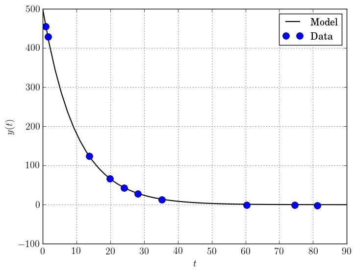
To generate this plot, run:
# Plot calibrated model vs. observations
ts = np.linspace(0.0, 90.0)
ys = soln.x[0] * np.exp(soln.x[1] * ts)

import matplotlib.pyplot as plt
plt.figure(1)
ax = plt.gca()  # current axes
ax.plot(ts, ys, 'k-', label='Model')
ax.plot(tdata, ydata, 'bo', label='Data')
ax.set_xlabel('t')
ax.set_ylabel('y(t)')
ax.legend(loc='upper right')
ax.grid()
plt.show()
Example: Solving a Nonlinear System of Equations
Lastly, we give an example of using DFO-LS to solve a nonlinear system of equations (taken from here). We wish to solve the following set of equations
The code for this is:
# DFO-LS example: Solving a nonlinear system of equations
# Originally from:
# http://support.sas.com/documentation/cdl/en/imlug/66112/HTML/default/viewer.htm#imlug_genstatexpls_sect004.htm

from __future__ import print_function
from math import exp
import numpy as np
import dfols

# Want to solve:
#   x1 + x2 - x1*x2 + 2 = 0
#   x1 * exp(-x2) - 1   = 0
def nonlinear_system(x):
    return np.array([x[0] + x[1] - x[0]*x[1] + 2,
                     x[0] * exp(-x[1]) - 1.0])

# Warning: if there are multiple solutions, which one
#          DFO-LS returns will likely depend on x0!
x0 = np.array([0.1, -2.0])

# Call DFO-LS
soln = dfols.solve(nonlinear_system, x0)

# Display output
print(soln)
The output of this is
****** DFO-LS Results ******
Solution xmin = [ 0.09777309 -2.32510588]
Residual vector = [-1.38601752e-09 -1.70204653e-08]
Objective value f(xmin) = 2.916172822e-16
Needed 13 objective evaluations (at 13 points)
Approximate Jacobian = [[ 3.32527052  0.90227531]
 [10.22943034 -0.99958226]]
Solution xmin was evaluation point 13
Approximate Jacobian formed using evaluation points [ 8 11 12]
Exit flag = 0
Success: Objective is sufficiently small
****************************
Here, we see that both entries of the residual vector are very small, so both equations have been solved to high accuracy.
References
Coralia Cartis, Jan Fiala, Benjamin Marteau and Lindon Roberts, Improving the Flexibility and Robustness of Model-Based Derivative-Free Optimization Solvers, ACM Transactions on Mathematical Software, 45:3 (2019), pp. 32:1-32:41 [preprint]
Matthew Hough and Lindon Roberts, Model-Based Derivative-Free Methods for Convex-Constrained Optimization, SIAM Journal on Optimization, 21:4 (2022), pp. 2552-2579 [preprint].
Yanjun Liu, Kevin H. Lam and Lindon Roberts, Black-box Optimization Algorithms for Regularized Least-squares Problems, arXiv preprint arXiv:2407.14915 (2024).
Jorge J. More, Burton S. Garbow and Kenneth E. Hillstrom, Testing Unconstrained Optimization Software, ACM Transactions on Mathematical Software, 7:1 (1981), pp. 17-41.