Using DFO-GN
This section describes the main interface to DFO-GN and how to use it.
How to use DFO-GN
The main interface to DFO-GN is via the function solve
soln = dfogn.solve(objfun, x0)
The input objfun is a Python function which takes an input \(x\in\mathbb{R}^n\) and returns the vector of residuals \([r_1(x)\: \cdots \: r_m(x)]\in\mathbb{R}^m\). Both the input and output of objfun must be one-dimensional NumPy arrays (i.e. with x.shape == (n,) and objfun(x).shape == (m,)).
The input x0 is the starting point for the solver, and (where possible) should be set to be the best available estimate of the true solution \(x_{min}\in\mathbb{R}^n\). It should be specified as a one-dimensional NumPy array (i.e. with x0.shape == (n,)).
As DFO-GN is a local solver, providing different values for x0 may cause it to return different solutions, with possibly different objective values.
Outputs
The output of dfogn.solve is an object soln containing:
soln.x- an estimate of the solution, \(x_{min}\in\mathbb{R}^n\), a one-dimensional NumPy array.soln.resid- the vector of residuals at the calculated solution \([r_1(x_{min})\: \cdots \: r_m(x_{min})]\in\mathbb{R}^m\)soln.f- the objective value at the calculated solution, \(f(x_{min})\), a Float.soln.jacobian- an estimate of the \(m\times n\) Jacobian matrix of first derivatives at the calculated solution \(J_{i,j} \approx \partial r_i(x_{min})/\partial x_j\), a two-dimensional NumPy array.soln.nf- the number of evaluations ofobjfunthat the algorithm needed, an Integer.soln.flag- an exit flag, which can take one of several values (listed below), an Integer.soln.msg- a description of why the algorithm finished, a String.
The possible values of flag are defined by the following variables, also defined in the soln object:
soln.EXIT_SUCCESS = 0- DFO-GN terminated successfully (the objective value or trust region radius are sufficiently small).soln.EXIT_INPUT_ERROR = 1- error in the inputs.soln.EXIT_MAXFUN_WARNING = 2- maximum allowed objective evaluations reached.soln.EXIT_TR_INCREASE_ERROR = 3- error occurred when solving the trust region subproblem.soln.EXIT_LINALG_ERROR = 4- linear algebra error, e.g. the interpolation points produced a singular linear system.soln.EXIT_ALTMOV_MEMORY_ERROR = 5- error occurred when determining a geometry-improving step.
For more information about how to interpret these descriptions, see the algorithm details section in Overview. If you encounter any of the last 4 conditions, first check to see if the output value is sufficient for your requirements, otherwise consider changing x0 or the optional parameter rhobeg (see below).
As variables are defined in the soln objected, they can be accessed with, for example
if soln.flag == soln.EXIT_SUCCESS:
    print("Success!")
Optional Arguments
The solve function has several optional arguments which the user may provide:
dfogn.solve(objfun, x0, lower=None, upper=None, maxfun=1000,
            rhobeg=None, rhoend=1e-8)
These arguments are:
lower- the vector \(a\) of lower bounds on \(x\) (default is \(a_i=-10^{20}\)).upper- the vector \(b\) of upper bounds on \(x\) (default is \(b_i=10^{20}\)).maxfun- the maximum number of objective evaluations the algorithm may request (default is 1000).rhobeg- the initial value of the trust region radius (default is \(0.1\max(\|x_0\|_{\infty}, 1)\)).rhoend- minimum allowed value of trust region radius, which determines when a successful termination occurs (default is \(10^{-8}\)).
There is a tradeoff when choosing the value of rhobeg: a large value allows the algorithm to progress to a solution quicker, but there is a greater risk that it tries points which do not reduce the objective. Similarly, a small value means a greater chance of reducing the objective, but potentially making slower progress towards the final solution.
The value of rhoend determines the level of accuracy desired in the solution xmin (smaller values give higher accuracy, but DFO-GN will take longer to finish).
The requirements on the inputs are:
Each entry of
lowermust be strictly below the corresponding entry ofupper, with a gap of at least twicerhobeg;Both
rhobegandrhoendmust be strictly positive, withrhoendbeing the smaller one; andThe value
maxfunmust be strictly positive, and generally should be abovelen(x)+1(which is the initial setup requirement).
A Simple Example
Suppose we wish to minimize the Rosenbrock function (a common test problem):
This function has only one local minimum \(f(x_{min})=0\) at \(x_{min}=(1,1)\). We can write this as a least-squares problem as:
A commonly-used starting point for testing purposes is \(x_0=(-1.2,1)\). The following script shows how to solve this problem using DFO-GN:
# DFO-GN example: minimize the Rosenbrock function
from __future__ import print_function
import numpy as np
import dfogn

# Define the objective function
def rosenbrock(x):
    return np.array([10.0 * (x[1] - x[0] ** 2), 1.0 - x[0]])

# Define the starting point
x0 = np.array([-1.2, 1.0])

# Call DFO-GN
soln = dfogn.solve(rosenbrock, x0)

# Display output
print(" *** DFO-GN results *** ")
print("Solution xmin = %s" % str(soln.x))
print("Objective value f(xmin) = %.10g" % soln.f)
print("Needed %g objective evaluations" % soln.nf)
print("Residual vector = %s" % str(soln.resid))
print("Approximate Jacobian = %s" % str(soln.jacobian))
print("Exit flag = %g" % soln.flag)
print(soln.msg)
The output of this script is
 *** DFO-GN results ***
Solution xmin = [ 1.  1.]
Objective value f(xmin) = 1.268313548e-17
Needed 50 objective evaluations
Residual vector = [ -3.56133900e-09   0.00000000e+00]
Approximate Jacobian = [[ -2.00012196e+01   1.00002643e+01]
 [ -1.00000000e+00   3.21018592e-13]]
Exit flag = 0
Success: Objective is sufficiently small
Note in particular that the Jacobian is not quite correct - the bottom-right entry should be exactly zero for all \(x\), for instance.
Adding Bounds and More Output
We can extend the above script to add constraints. To do this, we can add the lines
# Define bound constraints (a <= x <= b)
a = np.array([-10.0, -10.0])
b = np.array([0.9, 0.85])

# Call DFO-GN (with bounds)
soln = dfogn.solve(rosenbrock, x0, lower=a, upper=b)
DFO-GN correctly finds the solution to the constrained problem:
Solution xmin = [ 0.9   0.81]
Objective value f(xmin) = 0.01
Needed 44 objective evaluations
Residual vector = [ -2.01451078e-10   1.00000000e-01]
Approximate Jacobian = [[ -1.79999994e+01   1.00000004e+01]
 [ -9.99999973e-01   2.01450058e-08]]
Exit flag = 0
Success: rho has reached rhoend
However, we also get a warning that our starting point was outside of the bounds:
RuntimeWarning: Some entries of x0 above upper bound, adjusting
DFO-GN automatically fixes this, and moves \(x_0\) to a point within the bounds, in this case \(x_0=(-1.2, 0.85)\).
We can also get DFO-GN to print out more detailed information about its progress using the logging module. To do this, we need to add the following lines:
import logging
logging.basicConfig(level=logging.INFO, format='%(message)s')

# ... (call dfogn.solve)
And we can now see each evaluation of objfun:
Function eval 1 has f = 39.65 at x = [-1.2   0.85]
Function eval 2 has f = 14.337296 at x = [-1.08  0.85]
...
Function eval 43 has f = 0.010000000899913 at x = [ 0.9         0.80999999]
Function eval 44 has f = 0.01 at x = [ 0.9   0.81]
If we wanted to save this output to a file, we could replace the above call to logging.basicConfig() with
logging.basicConfig(filename="myfile.txt", level=logging.INFO,
                    format='%(message)s', filemode='w')
Example: Noisy Objective Evaluation
As described in Overview, derivative-free algorithms such as DFO-GN are particularly useful when objfun has noise. Let’s modify the previous example to include random noise in our objective evaluation, and compare it to a derivative-based solver:
# DFO-GN example: minimize the Rosenbrock function
from __future__ import print_function
import numpy as np
import dfogn

# Define the objective function
def rosenbrock(x):
    return np.array([10.0 * (x[1] - x[0] ** 2), 1.0 - x[0]])

# Modified objective function: add 1% Gaussian noise
def rosenbrock_noisy(x):
    return rosenbrock(x) * (1.0 + 1e-2 * np.random.normal(size=(2,)))

# Define the starting point
x0 = np.array([-1.2, 1.0])

# Set random seed (for reproducibility)
np.random.seed(0)

print("Demonstrate noise in function evaluation:")
for i in range(5):
    print("objfun(x0) = %s" % str(rosenbrock_noisy(x0)))
print("")

# Call DFO-GN
soln = dfogn.solve(rosenbrock_noisy, x0)

# Display output
print(" *** DFO-GN results *** ")
print("Solution xmin = %s" % str(soln.x))
print("Objective value f(xmin) = %.10g" % soln.f)
print("Needed %g objective evaluations" % soln.nf)
print("Residual vector = %s" % str(soln.resid))
print("Approximate Jacobian = %s" % str(soln.jacobian))
print("Exit flag = %g" % soln.flag)
print(soln.msg)

# Compare with a derivative-based solver
import scipy.optimize as opt
soln = opt.least_squares(rosenbrock_noisy, x0)

print("")
print(" *** SciPy results *** ")
print("Solution xmin = %s" % str(soln.x))
print("Objective value f(xmin) = %.10g" % (2.0 * soln.cost))
print("Needed %g objective evaluations" % soln.nfev)
print("Exit flag = %g" % soln.status)
print(soln.message)
The output of this is:
Demonstrate noise in function evaluation:
objfun(x0) = [-4.4776183   2.20880346]
objfun(x0) = [-4.44306447  2.24929965]
objfun(x0) = [-4.48217255  2.17849989]
objfun(x0) = [-4.44180389  2.19667014]
objfun(x0) = [-4.39545837  2.20903317]

 *** DFO-GN results ***
Solution xmin = [ 1.  1.]
Objective value f(xmin) = 4.658911493e-15
Needed 56 objective evaluations
Residual vector = [ -6.82177042e-08  -2.29266787e-09]
Approximate Jacobian = [[ -2.01345344e+01   1.01261457e+01]
 [ -1.00035048e+00  -5.99847638e-03]]
Exit flag = 0
Success: Objective is sufficiently small

 *** SciPy results ***
Solution xmin = [-1.20000033  1.00000016]
Objective value f(xmin) = 23.66957245
Needed 6 objective evaluations
Exit flag = 3
`xtol` termination condition is satisfied.
DFO-GN is able to find the solution with only 6 more function evaluations than in the noise-free case. However SciPy’s derivative-based solver, which has no trouble solving the noise-free problem, is unable to make any progress.
Example: Parameter Estimation/Data Fitting
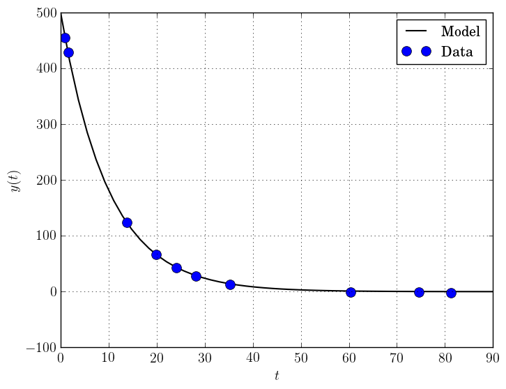
Next, we show a short example of using DFO-GN to solve a parameter estimation problem (taken from here). Given some observations \((t_i,y_i)\), we wish to calibrate parameters \(x=(x_1,x_2)\) in the exponential decay model
The code for this is:
# DFO-GN example: data fitting problem
# Originally from:
# https://uk.mathworks.com/help/optim/ug/lsqcurvefit.html
from __future__ import print_function
import numpy as np
import dfogn

# Observations
tdata = np.array([0.9, 1.5, 13.8, 19.8, 24.1, 28.2, 35.2,
                  60.3, 74.6, 81.3])
ydata = np.array([455.2, 428.6, 124.1, 67.3, 43.2, 28.1, 13.1,
                  -0.4, -1.3, -1.5])

# Model is y(t) = x[0] * exp(x[1] * t)
def prediction_error(x):
    return ydata - x[0] * np.exp(x[1] * tdata)

# Define the starting point
x0 = np.array([100.0, -1.0])

# We expect exponential decay: set upper bound x[1] <= 0
upper = np.array([1e20, 0.0])

# Call DFO-GN
soln = dfogn.solve(prediction_error, x0, upper=upper)

# Display output
print(" *** DFO-GN results *** ")
print("Solution xmin = %s" % str(soln.x))
print("Objective value f(xmin) = %.10g" % soln.f)
print("Needed %g objective evaluations" % soln.nf)
print("Exit flag = %g" % soln.flag)
print(soln.msg)
The output of this is (noting that DFO-GN moves \(x_0\) to be far away enough from the upper bound)
RuntimeWarning: Some entries of x0 too close to upper bound, adjusting
 *** DFO-GN results ***
Solution xmin = [  4.98830861e+02  -1.01256863e-01]
Objective value f(xmin) = 9.504886892
Needed 107 objective evaluations
Exit flag = 0
Success: rho has reached rhoend
This produces a good fit to the observations.
Example: Solving a Nonlinear System of Equations
Lastly, we give an example of using DFO-GN to solve a nonlinear system of equations (taken from here). We wish to solve the following set of equations
The code for this is:
# DFO-GN example: Solving a nonlinear system of equations
# http://support.sas.com/documentation/cdl/en/imlug/66112/HTML/default/viewer.htm#imlug_genstatexpls_sect004.htm

from __future__ import print_function
import math
import numpy as np
import dfogn

# Want to solve:
#   x1 + x2 - x1*x2 + 2 = 0
#   x1 * exp(-x2) - 1   = 0
def nonlinear_system(x):
    return np.array([x[0] + x[1] - x[0]*x[1] + 2,
                     x[0] * math.exp(-x[1]) - 1.0])

# Warning: if there are multiple solutions, which one
#          DFO-GN returns will likely depend on x0!
x0 = np.array([0.1, -2.0])

soln = dfogn.solve(nonlinear_system, x0)

# Display output
print(" *** DFO-GN results *** ")
print("Solution xmin = %s" % str(soln.x))
print("Objective value f(xmin) = %.10g" % soln.f)
print("Needed %g objective evaluations" % soln.nf)
print("Residual vector = %s" % str(soln.resid))
print("Exit flag = %g" % soln.flag)
print(soln.msg)
The output of this is
 *** DFO-GN results ***
Solution xmin = [ 0.09777309 -2.32510588]
Objective value f(xmin) = 2.916172822e-16
Needed 13 objective evaluations
Residual vector = [ -1.38601752e-09  -1.70204653e-08]
Exit flag = 0
Success: Objective is sufficiently small
Here, we see that both entries of the residual vector are very small, so both equations have been solved to high accuracy.